State Space Model Forecasting

Produces forecasts using a fitted State Space Model.

StateSpaceForecast(
  fit,
  addvar_list_fc = NULL,
  level_addvar_list_fc = NULL,
  self_spec_list_fc = NULL,
  forecast_period = 1
)

Arguments

fit	A list containing the specifications of the State Space Model, as returned by StateSpaceFit or StateSpaceEval.
addvar_list_fc	A list containing the explanatory variables for each of the dependent variables. The list should contain p (number of dependent variables) elements. Each element of the list should be a forecast_period x k_p matrix, with k_p being the number of explanatory variables for the pth dependent variable. If no explanatory variables should be added for one of the dependent variables, then set the corresponding element to NULL.
level_addvar_list_fc	A list containing the explanatory variables for each of the dependent variables. The list should contain p (number of dependent variables) elements. Each element of the list should be a forecast_period x k_p matrix, with k_p being the number of explanatory variables for the pth dependent variable. If no explanatory variables should be added for one of the dependent variables, then set the corresponding element to NULL.
self_spec_list_fc	A list containing the specification of the self specified component. Does not have to be specified if it does not differ from self_spec_list as passed on to StateSpaceFit() or StateSpaceEval(). If some system matrices are time-varying then you should specify this argument. See StateSpaceFit() for details about the format that must be followed for this argument.
forecast_period	Number of time steps to forecast ahead.

Value

A list containing the forecasts and corresponding uncertainties. In addition, it returns the components of the forecasts, as specified by the State Space model.

References

Durbin J, Koopman SJ (2012). Time series analysis by state space methods. Oxford university press.

Examples

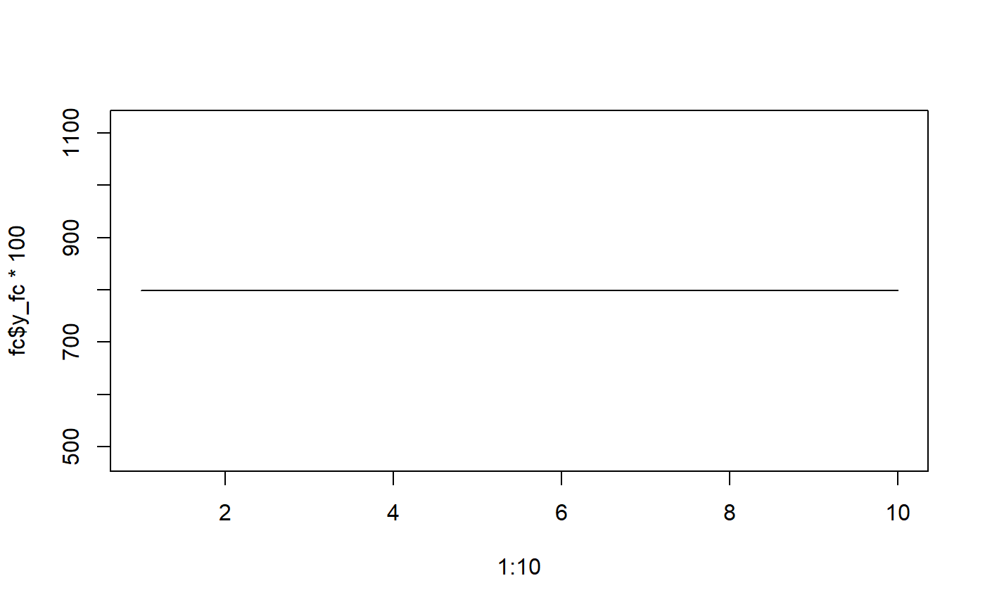
# Fits a local level model for the Nile data
library(datasets)
y <- matrix(Nile)
fit <- StateSpaceFit(initial = 1, y = y / 100, local_level_ind = TRUE)
#> Warning: Number of initial parameters is less than the required amount of parameters (2), recycling the initial parameters the required amount of times.
#> Starting the optimisation procedure at: 2020-05-08 23:18:43
#> Parameter scaling:[1] 1 1
#> initial  value 2.443183 
#> iter  10 value 1.775548
#> final  value 1.775527 
#> converged
#> Finished the optimisation procedure at: 2020-05-08 23:18:44
#> Time difference of 0.603209972381592 secs

# Obtain forecasts for 10 steps ahead using the fitted model
fc <- StateSpaceForecast(fit, forecast_period = 10)

# Plot the forecasts
plot(1:10, fc$y_fc * 100, type = 'l')